The GPU Memory Wall: Forecasting AI Demand to 2028
Memory is the new compute bottleneck. Here is where we are, where we are headed, and what organizations should do before it is too late.
Introduction: Memory Is the New Compute
For years, the AI hardware conversation centered on compute: teraflops, tensor cores, and training throughput. That conversation is now obsolete. The defining constraint of modern AI infrastructure is not how fast you can multiply matrices; it is whether you can fit the model in memory at all.
Every major operational failure in production AI serving traces back to memory. Out-of-memory crashes during traffic spikes. Degraded throughput because KV caches bloated beyond capacity. Entire model deployments re-architected because a context window extension doubled VRAM requirements overnight. Compute is abundant and getting cheaper. Memory is scarce, expensive, and getting worse.
This post presents a comprehensive, data-driven analysis of GPU memory demand through 2028. We cover the current landscape, the technologies on the roadmap, the supply chain constraints that will gate availability, and the concrete strategies that engineering teams should adopt right now. All memory calculations referenced in this piece can be reproduced using the InferenceBench GPU Inference Calculator.
Where We Are: The 2025-2026 Memory Landscape
To understand where we are going, we need an honest assessment of where we stand. As of mid-2026, the GPU memory landscape for AI inference and training looks like this:
| GPU | Memory | HBM Generation | Bandwidth | Street Price (approx.) | $/GB |
|---|---|---|---|---|---|
| NVIDIA A100 | 80 GB | HBM2e | 2.0 TB/s | $12,000-15,000 | $150-188 |
| NVIDIA H100 SXM | 80 GB | HBM3 | 3.35 TB/s | $25,000-30,000 | $312-375 |
| NVIDIA H200 | 141 GB | HBM3e | 4.8 TB/s | $30,000-35,000 | $213-248 |
| NVIDIA B200 | 192 GB | HBM3e | 8.0 TB/s | $35,000-40,000 | $182-208 |
| NVIDIA B300 (projected) | 288 GB | HBM3e (12-Hi) | 8.0+ TB/s | $40,000-50,000 | $139-174 |
| AMD MI300X | 192 GB | HBM3 | 5.3 TB/s | $12,000-15,000 | $63-78 |
| AMD MI325X | 256 GB | HBM3e | 6.0 TB/s | $15,000-20,000 | $59-78 |
The H100 remains the workhorse of production inference. With 80 GB of HBM3, it can serve models up to roughly 40 billion parameters at FP16 precision, or up to 80 billion parameters with INT8 quantization. For the models that dominate production traffic today (Llama 3.1 70B, Mixtral 8x22B, GPT-4 class models), an H100 is often memory-constrained before it is compute-constrained. You run out of VRAM for your KV cache before you saturate the tensor cores.
The H200, with 141 GB of HBM3e and 4.8 TB/s bandwidth, was the first GPU to seriously address this gap. It allows comfortable serving of 70B-class models with generous batch sizes and longer context windows. But even the H200 hits a wall with 400B+ parameter models. Serving Llama 4 Maverick (400B parameters, MoE) on a single H200 is not feasible at full precision; you need either quantization or multi-GPU tensor parallelism.
The B200 and its projected successor B300 represent significant steps forward. At 192 GB and 288 GB respectively, they bring single-GPU memory into the range where many frontier models become servable without aggressive quantization. But as we will show, model growth is outpacing memory growth.
Why Memory Demand Is Accelerating
GPU memory demand is driven by four compounding forces, each growing on its own exponential curve. Together, they create a demand trajectory that is steeper than any single factor suggests.
1. Model Parameter Growth
The trend in frontier model size is well-documented but worth restating with current data:
| Model | Release | Parameters | FP16 Weight Memory |
|---|---|---|---|
| GPT-3 | June 2020 | 175B | 350 GB |
| PaLM | April 2022 | 540B | 1,080 GB |
| GPT-4 (estimated) | March 2023 | ~1,800B (MoE) | ~3,600 GB |
| DeepSeek V3 | December 2024 | 671B (MoE) | 1,342 GB |
| Llama 4 Maverick | April 2025 | 400B (MoE) | 800 GB |
The compound growth rate of frontier model parameters has averaged roughly 4x every two years since 2020. While the shift toward Mixture-of-Experts (MoE) architectures means that active parameters per token are lower, the total weight footprint that must reside in memory remains large. A 671B MoE model that activates only 37B parameters per token still requires the full 671B parameter set loaded into GPU memory (or accessible via fast memory tiers). MoE saves compute, not memory.
2. Context Window Explosion
Context window growth has been even more dramatic than parameter growth:
| Year | Typical Context Window | Notable Models |
|---|---|---|
| 2022 | 2K-4K tokens | GPT-3.5, early LLMs |
| 2023 | 4K-32K tokens | GPT-4 (8K/32K), Claude 2 (100K) |
| 2024 | 128K-200K tokens | GPT-4 Turbo (128K), Claude 3 (200K), Gemini 1.5 Pro (1M) |
| 2025 | 200K-1M+ tokens | Claude 3.5 (200K), Gemini 2.0 (2M), MiniMax M2.7 (1M) |
| 2026 | 1M-10M tokens (projected) | Research models pushing 10M+ context |
This matters because the KV cache, the data structure that stores the key-value pairs for the attention mechanism, scales linearly with both sequence length and batch size. For a model like Llama 3.1 70B with a 128K context window serving a batch of 16 requests, the KV cache alone can consume 40-60 GB of VRAM. At 1M context, that number balloons to 300+ GB, dwarfing the weight memory. The context window, not the model weights, is the primary memory consumer in long-context serving.
3. Multi-Modal Models
The shift from text-only to multi-modal models introduces additional memory demands that are often underestimated:
- Vision encoders: Models like GPT-4V, LLaVA, and Gemini include vision transformers (ViT) that add 300M-6B parameters and require separate activation memory for image processing.
- Image token expansion: A single 1024x1024 image can expand to 576-2048 tokens in the LLM context, consuming KV cache space equivalent to hundreds of text tokens.
- Audio processing: Real-time speech models (GPT-4o, Gemini Live) require continuous audio buffer memory and streaming attention caches.
- Cross-modal attention: Fusing modalities requires additional attention heads and associated KV cache entries.
A multi-modal model serving mixed image-text workloads can require 30-50% more memory than the same parameter-count text-only model, depending on image resolution and the ratio of visual to textual content.
4. Batch Serving Economics
Production serving is not about running one request at a time. To achieve reasonable GPU utilization and cost efficiency, inference servers batch multiple requests together. Each request in the batch requires its own KV cache allocation. The economics are ruthless:
- At batch size 1, GPU utilization might be 10-20% because inference is memory-bandwidth-bound, not compute-bound.
- At batch size 32-64, utilization rises to 60-80%, but KV cache memory scales linearly with batch size.
- The optimal batch size is determined by whichever runs out first: compute or memory. In 2026, it is almost always memory.
This creates a direct economic link between GPU memory and cost-per-token. More memory means larger batches, higher utilization, and lower cost per token. Memory is not just a technical constraint; it is a unit economics lever.
The Memory Math: Calculating VRAM for a Modern Model
Understanding GPU memory demand requires knowing the formula. There is nothing mysterious about it: inference memory consumption is the sum of three components, each of which can be calculated from model architecture parameters. You can verify all of these calculations using the InferenceBench GPU Inference Calculator.
Total Inference VRAM = Weights + KV Cache + Activations + Overhead
1. Model Weights
Weight Memory (GB) = (Parameters x Bytes per Parameter) / (1024^3)

Examples:
  Llama 3.1 70B at FP16:  70B x 2 bytes  = 140 GB
  Llama 3.1 70B at INT8:  70B x 1 byte   = 70 GB
  Llama 3.1 70B at INT4:  70B x 0.5 byte  = 35 GB
  DeepSeek V3 671B at FP16: 671B x 2 bytes = 1,342 GB
2. KV Cache
KV Cache (GB) = 2 x Layers x Heads_KV x Head_Dim x Seq_Len x Batch_Size x Bytes_per_Element / (1024^3)

Where:
  2           = one K tensor + one V tensor
  Layers      = number of transformer layers (e.g., 80 for Llama 3.1 70B)
  Heads_KV    = number of KV heads (8 for GQA in Llama 3.1 70B)
  Head_Dim    = dimension per head (128 typical)
  Seq_Len     = context window length in tokens
  Batch_Size  = concurrent requests
  Bytes       = 2 for FP16, 1 for INT8 KV cache

Example: Llama 3.1 70B, 128K context, batch 16, FP16 KV cache:
  2 x 80 x 8 x 128 x 131,072 x 16 x 2 = ~53.7 GB
This is the number that surprises most people. The KV cache for a 70B model at moderate batch sizes and long context can rival or exceed the weight memory itself. At 1M context, the KV cache dominates everything.
3. Activations and Runtime Overhead
Activation Memory = ~5-15% of weight memory (during inference, much higher during training)
Runtime Overhead   = CUDA context (~500 MB) + framework buffers (~1-3 GB)
Safety Margin      = 5-10% of total for memory fragmentation
Putting It Together: Real-World Example
Let us walk through a realistic production scenario: serving Llama 3.1 70B at INT8 precision with a 32K context window and a batch size of 32.
| Component | Calculation | Memory |
|---|---|---|
| Weights (INT8) | 70B x 1 byte | 70.0 GB |
| KV Cache (FP16) | 2 x 80 x 8 x 128 x 32,768 x 32 x 2 bytes | 26.8 GB |
| Activations | ~10% of weights | 7.0 GB |
| Runtime overhead | CUDA context + buffers | 3.0 GB |
| Fragmentation margin | ~5% | 5.3 GB |
| Total | 112.1 GB |
This deployment does not fit on a single H100 (80 GB). It fits on an H200 (141 GB) with 29 GB headroom. On a B200 (192 GB), you have 80 GB of headroom, which means you could increase the batch size to ~80 or extend the context window to 128K. Memory directly translates to serving capacity.
Experiment with these calculations yourself at inferencebench.io/calculator, where you can adjust model parameters, precision, context length, and batch size interactively.
Memory Technology Roadmap: HBM3e to HBM4 to HBM4E
GPU memory capacity is ultimately gated by High Bandwidth Memory (HBM) technology. Understanding the HBM roadmap is essential for forecasting what will be possible, and what will remain constrained, over the next three years.
HBM Generations: Specifications and Timeline
| Generation | Stack Height | Capacity per Stack | Bandwidth per Stack | Max per GPU (typical) | Production Status |
|---|---|---|---|---|---|
| HBM3 | 8-Hi | 16 GB | ~820 GB/s | 80 GB (5 stacks) | Volume production |
| HBM3e (8-Hi) | 8-Hi | 24 GB | ~1.2 TB/s | 141 GB (6 stacks, H200) | Volume production |
| HBM3e (12-Hi) | 12-Hi | 36 GB | ~1.2 TB/s | 192 GB (B200), 288 GB (B300 projected) | Ramping 2025-2026 |
| HBM4 (SK Hynix) | 12-Hi (projected) | 48 GB (projected) | ~1.5+ TB/s | 288-384 GB (projected) | Sampling late 2026, volume 2027 |
| HBM4E | 16-Hi (projected) | 64 GB (projected) | ~2.0 TB/s | 384-512 GB (projected) | Projected 2028 |
Sources: SK Hynix HBM roadmap presentations (2024-2025), Samsung HBM4 announcements, NVIDIA GTC 2025, TrendForce DRAM market reports, Yole Developpement HBM market forecast.
Key Observations
Capacity is growing, but not as fast as demand. HBM capacity per GPU is roughly doubling every two years: 80 GB (H100, 2023) to 141 GB (H200, 2024) to 192 GB (B200, 2025) to a projected 288-384 GB (next-gen, 2027). That is approximately 2x per generation on a 18-24 month cycle. Model memory requirements, as shown earlier, are growing at 4x every two years. The gap is widening.
Bandwidth growth is keeping pace, barely. HBM bandwidth has grown from 2.0 TB/s (A100) to 3.35 TB/s (H100) to 4.8 TB/s (H200) to 8.0 TB/s (B200). This matters because inference is bandwidth-bound: the time to generate each token is dominated by reading model weights from memory. If capacity doubles but bandwidth does not keep pace, you have more memory you cannot feed to the compute units fast enough. The B200's 8 TB/s represents a genuine step change.
Cost per GB is improving slowly. HBM remains the most expensive memory technology in the stack. Industry estimates from TrendForce and Yole Developpement place HBM3e costs at $25-40 per GB at the chip level, before integration into a GPU package. HBM4 is projected to initially cost 30-50% more per GB before manufacturing efficiencies bring it down. For a 384 GB GPU, that is $9,600-15,360 in HBM alone, representing 30-40% of the total GPU bill of materials.
The HBM4 Transition
HBM4 represents a significant architectural change. Unlike HBM3/HBM3e, which use a standardized interface across manufacturers, HBM4 adopts a customizable base logic die that can be tailored to specific processor architectures. SK Hynix has confirmed that initial HBM4 products will target NVIDIA's next-generation GPU platform (likely the "Rubin" architecture expected in 2027).
Key projected improvements in HBM4:
- Bandwidth: 6-8 TB/s per stack, with a per-pin data rate of 6.4 Gbps (vs. 4.8 Gbps for HBM3e), according to JEDEC preliminary specifications.
- Capacity: 48-64 GB per stack (12-Hi to 16-Hi), potentially yielding 288-512 GB per GPU.
- Energy efficiency: 30% reduction in energy per bit transferred, per SK Hynix projections.
- Custom logic die: The base die can include processing-in-memory capabilities, potentially offloading simple operations closer to the data.
Samsung has announced its own HBM4 roadmap, targeting volume production in 2027 with a competitive specification. The company is emphasizing its 3D packaging expertise and hybrid bonding technology as differentiators.
Supply Chain Reality: The HBM Bottleneck
Understanding HBM supply dynamics is critical for anyone planning GPU procurement. The supply chain is concentrated, capacity-constrained, and exposed to significant geopolitical risk.
Market Concentration
The global HBM market is an oligopoly with three producers:
- SK Hynix: ~50-53% market share (2025), dominant supplier to NVIDIA. Based in Icheon, South Korea, with major fab operations in South Korea and a facility in Wuxi, China.
- Samsung: ~38-40% market share (2025), recovering from yield issues that delayed HBM3e qualification. Based in Hwaseong, South Korea.
- Micron: ~8-10% market share (2025), a distant third but growing. Based in Boise, Idaho, with manufacturing in Hiroshima, Japan and Singapore.
Source: TrendForce Q1 2025 HBM market report, Yole Developpement Memory Market Monitor.
Manufacturing Constraints
HBM is not simply "more DRAM." Manufacturing HBM requires:
- 2-3x more wafer area per GB compared to standard DDR5, because HBM dies are physically larger and yield-sensitive.
- Advanced packaging: Each HBM stack requires through-silicon vias (TSVs), micro-bumps, and wafer-level testing, processes that add cost and reduce throughput compared to conventional DRAM packaging.
- Hybrid bonding (for HBM4): Next-generation HBM stacks will require hybrid copper-to-copper bonding, a technology currently ramping at TSMC, SK Hynix, and Samsung. Yield rates for 12-Hi and 16-Hi stacks using hybrid bonding are still being optimized.
- Dedicated fab capacity: Converting a DRAM production line to HBM production is a multi-quarter process. Manufacturers face a tradeoff: every wafer allocated to HBM is a wafer not producing higher-volume commodity DRAM.
TrendForce estimates that HBM consumed approximately 5-6% of total DRAM wafer capacity in 2025, projected to reach 8-10% by 2027. This sounds small, but it represents a disproportionate share of advanced-node capacity and packaging resources.
Lead Times and Procurement
Current lead times for HBM-equipped GPUs reflect the compounding constraints:
- H100/H200 servers: 3-6 months (improving as B200 absorbs demand).
- B200 systems: 6-12 months (strong demand, ramping production).
- B300/next-gen: 12-18+ months (pre-orders being taken, delivery timelines uncertain).
- Custom HBM configurations: Hyperscaler-volume orders (10,000+ GPU commitments) receive priority allocation; smaller customers face longer waits.
The practical implication is straightforward: if your organization determines in Q3 2026 that it needs next-generation GPU capacity, the hardware may not arrive until Q1-Q3 2028. Planning horizons for GPU memory capacity need to extend 18-24 months, minimum.
Geopolitical Risk
The HBM supply chain is concentrated in a geopolitically sensitive region. SK Hynix and Samsung, representing ~90% of HBM production, are both headquartered in South Korea. Their advanced packaging operations are located in South Korea, with some assembly in China. Key considerations:
- Taiwan Strait: TSMC provides advanced packaging services (CoWoS) critical to integrating HBM into GPU packages. Any disruption to TSMC operations would cascade through the entire AI hardware supply chain.
- Korean Peninsula: While not a new risk, the concentration of HBM manufacturing on the Korean Peninsula means that regional instability would affect a majority of the world's HBM supply.
- US-China trade restrictions: Export controls on advanced AI chips and HBM to China have reduced the addressable market for SK Hynix and Samsung, potentially affecting production economics and R&D investment decisions.
- Japan: Micron's Hiroshima fab provides some geographic diversification, and the Japanese government has invested heavily in semiconductor manufacturing incentives.
No amount of software optimization can substitute for hardware that does not exist. Supply chain awareness must be part of any serious GPU memory planning exercise.
Forecasting 2026-2028: Where the Numbers Go
Based on the growth trends in model size, context length, multi-modal requirements, and batch serving economics, we can project memory demand against available supply for the next three years. These projections are necessarily approximate and are intended to illustrate the direction and magnitude of the gap.
Methodology
We model memory demand across three tiers: frontier models (the largest, most capable models from leading labs), production models (the models most commonly deployed in production inference), and efficient models (smaller models optimized for cost-effective serving). For each tier, we project weight memory, KV cache requirements at representative batch sizes and context lengths, and the resulting per-GPU memory demand at common precision levels.
Demand Projections
| Category | Metric | 2025 (Actual) | 2026 (Est.) | 2027 (Projected) | 2028 (Projected) |
|---|---|---|---|---|---|
| Frontier model size | Total parameters | 1-2T (MoE) | 2-4T (MoE) | 4-8T (MoE) | 8-16T (MoE) |
| Frontier model | FP16 weight memory | 2-4 TB | 4-8 TB | 8-16 TB | 16-32 TB |
| Production model size | Total parameters | 70-400B | 100-600B | 200B-1T | 400B-2T |
| Production model | INT4 weight memory | 35-200 GB | 50-300 GB | 100-500 GB | 200 GB-1 TB |
| Context window | Standard | 128K-1M | 256K-2M | 512K-4M | 1M-10M |
| KV cache per request | At standard context | 0.5-4 GB | 1-8 GB | 2-16 GB | 4-32 GB |
| Batch size (target) | For cost efficiency | 32-64 | 64-128 | 128-256 | 256-512 |
| Per-GPU memory need | Production tier, INT4 | 80-192 GB | 150-300 GB | 250-500 GB | 400 GB-1 TB |
| Available per GPU | Top-end HBM | 192 GB (B200) | 288 GB (B300) | 288-384 GB (HBM4) | 384-512 GB (HBM4E) |
Note: Frontier model sizes and context window projections are based on extrapolation from 2020-2025 growth rates, cross-referenced with published research roadmaps. Actual values will depend on architectural innovations, scaling law discoveries, and economic constraints. Projections should be treated as directional, not precise.
The Widening Gap
The table above reveals a structural problem. In 2025, the top-end GPU (B200, 192 GB) could barely accommodate the production tier at full batch size. By 2027, even with HBM4 delivering 288-384 GB per GPU, the memory demand for production-tier models at efficient batch sizes is projected to reach 250-500 GB. By 2028, the gap between demand and single-GPU capacity is projected to widen further.
This means that multi-GPU serving is the default, not the exception. Tensor parallelism across 2-8 GPUs will be required for most production models by 2027-2028. The implication for infrastructure cost is significant: memory constraints force you to provision 2-4x more GPUs than compute alone would require.
Total Market Memory Demand
Looking at aggregate demand, industry analysts project the following:
- 2025: ~40 million HBM units shipped (est.), representing ~4.8 exabytes of HBM capacity deployed globally (TrendForce).
- 2026: ~65-80 million HBM units projected, as B200/B300 ramp and data center expansion continues.
- 2027-2028: HBM revenue projected to exceed $100 billion annually (Yole Developpement), driven by AI accelerator demand.
Even with this massive production ramp, demand is projected to outstrip supply. TrendForce projects HBM supply shortages persisting through at least 2027, with allocation priority going to hyperscalers and large enterprise customers.
Strategies to Beat the Memory Wall
If raw HBM capacity cannot keep pace with model growth, the industry must find ways to do more with less. Fortunately, significant progress has been made on multiple fronts. These are the strategies that matter most, ranked by practical impact.
1. Quantization: The Single Biggest Lever
Quantization, reducing the numerical precision of model weights and activations, remains the most impactful memory reduction technique. The state of the art in 2026:
| Precision | Bytes per Param | Memory Reduction vs. FP16 | Quality Impact | Maturity |
|---|---|---|---|---|
| FP16/BF16 | 2.0 | Baseline | None | Standard |
| INT8 (W8A8) | 1.0 | 2x | Minimal (<1% on MMLU) | Production-ready |
| INT4 (W4A16) | 0.5 | 4x | Small (1-3% on MMLU) | Production-ready (GPTQ, AWQ) |
| INT4 (W4A4) | 0.5 | 4x (weights and activations) | Moderate (2-5% on MMLU) | Emerging (QuaRot, QServe) |
| INT3/NF3 | 0.375 | 5.3x | Moderate-significant | Research |
| INT2 (w/ outlier handling) | 0.25 | 8x | Significant (requires calibration) | Research |
The practical recommendation is clear: INT4 quantization (GPTQ or AWQ) should be the default for production inference in 2026. The quality-memory tradeoff is overwhelmingly favorable for most applications. A 70B model at INT4 requires 35 GB of weight memory instead of 140 GB, the difference between a single H100 and four H100s. Evaluate the quality-precision tradeoffs for your specific model using the InferenceBench precision comparison tool.
2. Mixture-of-Experts: Compute Efficiency, Not Memory Efficiency
MoE architectures (DeepSeek V3, Mixtral, Llama 4 Maverick) activate only a subset of parameters per token, typically 10-40% of total parameters. This dramatically reduces compute per token but does not reduce memory proportionally, because all expert weights must be resident in memory (or in a fast-accessible memory tier) to handle routing decisions.
That said, MoE does provide an indirect memory benefit: because compute per token is lower, you can afford to use more aggressive quantization without hitting compute bottlenecks. A 671B MoE model at INT4 requires ~168 GB of weight memory and activates only ~37B parameters per token, achieving quality comparable to a 200B dense model while fitting in a more reasonable memory envelope.
The takeaway: MoE is a compute strategy with memory implications, not a memory strategy. It is best combined with quantization.
3. KV Cache Optimization: Where the Real Innovation Is Happening
Since KV cache is the fastest-growing memory consumer, optimizations targeting the KV cache have outsized impact:
- Grouped-Query Attention (GQA): Reduces KV heads by 4-8x compared to Multi-Head Attention (MHA). Llama 3.1 70B uses 8 KV heads vs. 64 attention heads, reducing KV cache by 8x. This is now standard in all major model architectures.
- Multi-Query Attention (MQA): Takes GQA to the extreme with a single KV head. Used in some specialized models. Reduces KV cache by the number of attention heads (e.g., 64x for a 64-head model). Quality impact can be significant for complex tasks.
- PagedAttention (vLLM): Manages KV cache like virtual memory pages, eliminating fragmentation and enabling near-100% memory utilization. Reduces effective KV cache overhead by 20-40% compared to naive allocation. This is production-standard in 2026.
- Sliding Window Attention: Limits attention to a fixed window of recent tokens plus a global attention set. Used in Mistral and some Gemini variants. Caps KV cache growth at a fixed maximum regardless of context length. Tradeoff: reduced ability to reference distant context.
- KV Cache Compression: INT8 or INT4 quantization of KV cache values (separate from weight quantization). Can reduce KV cache memory by 2-4x with minimal quality impact. Increasingly supported by inference engines like TensorRT-LLM and vLLM.
- Token Eviction / Pruning: Dynamically evicting low-attention KV entries from the cache. Research techniques like H2O (Heavy-Hitter Oracle) and ScissorHands show promising results, reducing KV cache by 50-90% for certain workloads.
4. Disaggregated Serving: Splitting Prefill and Decode
A significant architectural innovation gaining production adoption is disaggregated serving, separating the prefill phase (processing the input prompt) from the decode phase (generating output tokens).
Prefill is compute-intensive: processing thousands of input tokens in parallel. Decode is memory-bandwidth-intensive: generating one token at a time, reading the entire model from memory for each token. These phases have fundamentally different hardware requirements.
By running prefill on compute-optimized GPUs and decode on memory-optimized GPUs (or even CXL-attached memory pools), operators can independently scale each resource. DistServe (from Peking University/Microsoft Research), Splitwise (from Microsoft), and NVIDIA's TensorRT-LLM with disaggregated mode all implement variants of this approach.
Early production deployments report 30-60% improvements in cost efficiency compared to monolithic serving, primarily because decode GPUs can be provisioned with more memory and less compute.
5. CXL Memory Pooling: Extending Beyond On-Die HBM
Compute Express Link (CXL) is an emerging interconnect standard that allows GPUs to access memory beyond their on-die HBM through a high-speed, cache-coherent interface. CXL 2.0 and 3.0 enable:
- Memory expansion: Attaching additional DRAM (DDR5) to a GPU via CXL, creating a "near memory" tier between HBM and system memory.
- Memory pooling: Sharing a pool of CXL-attached memory across multiple GPUs, dynamically allocating memory to whichever GPU needs it most.
- Tiered memory: Storing model weights in HBM and KV cache overflow in CXL-attached DRAM, accepting the bandwidth penalty (CXL DDR5: ~100 GB/s vs. HBM3e: ~4.8 TB/s) for less frequently accessed data.
CXL memory is not a replacement for HBM; it is a complement. The bandwidth gap (roughly 40-80x slower than HBM) means it is unsuitable for hot data paths like weight reads during token generation. But for KV cache spill, infrequently accessed expert weights in MoE models, and prefill-phase computations, CXL memory can meaningfully extend the effective memory capacity of a GPU system.
Samsung, SK Hynix, and Micron have all announced CXL memory products. NVIDIA's NVLink and NVSwitch fabrics are expected to integrate CXL support in future generations. We project CXL memory pooling will be a standard feature of data center GPU deployments by 2027-2028.
6. Model Distillation: Smaller Models, Preserved Quality
Distillation, training a smaller "student" model to mimic the outputs of a larger "teacher" model, remains one of the most effective ways to reduce memory requirements for production workloads. Notable examples:
- Llama 3.1 8B distilled from larger Llama models achieves performance competitive with 2023-era 70B models on many benchmarks.
- DeepSeek R1 distilled variants (1.5B, 7B, 14B) retain significant reasoning capability from the full 671B model.
- Phi-4 (14B) from Microsoft achieves quality competitive with much larger models through careful data curation and distillation.
Distillation is not a technology per se; it is a workflow. The key insight is that for many production use cases, the full capability of a frontier model is not needed. A well-distilled smaller model can serve 80-90% of production traffic at a fraction of the memory cost, with the frontier model reserved for the hardest queries.
What Smart Teams Are Doing Now
Based on our conversations with infrastructure teams at enterprises and cloud providers, here is what the most forward-thinking organizations are doing today to prepare for the memory wall.
1. Inventorying Current Memory Utilization
You cannot optimize what you do not measure. The first step is understanding your current memory consumption across all deployed models. Key metrics to track:
- Peak VRAM utilization per GPU (not average; memory is a peak-resource problem).
- KV cache utilization as a percentage of total available memory.
- Memory fragmentation ratio (actual used vs. allocated).
- Batch size achieved vs. theoretical maximum at current memory.
Use InferenceBench to model these metrics for your model portfolio and identify which deployments are memory-constrained.
2. Evaluating Quantization Across Their Model Portfolio
Every model in production should have a quantization evaluation: what precision is it running at, what precision could it run at, and what is the quality-memory tradeoff? Many teams discover that INT4 quantization gives them 2-3x more batch capacity with negligible quality regression for their specific use case.
3. Adopting Memory-Efficient Architectures
When selecting new models for deployment, memory efficiency should be a primary criterion alongside quality and latency. Prefer models with GQA over MHA. Prefer MoE architectures when the quality-to-memory ratio is favorable. Prefer architectures designed for KV cache efficiency (sliding window, sparse attention).
4. Planning GPU Procurement 18-24 Months Out
Given lead times, organizations that need next-generation GPU capacity in 2028 should be initiating conversations with cloud providers and GPU vendors today. This includes:
- Establishing reserved instance commitments with cloud providers for B200/B300 capacity.
- Evaluating colocation and on-premise options for guaranteed access.
- Diversifying across NVIDIA and AMD to reduce single-vendor dependency.
Use the InferenceBench Workload Matcher to determine the optimal GPU configuration for your projected 2027-2028 workloads, factoring in model growth and context window expansion.
5. Building Memory-Aware Infrastructure
Infrastructure decisions made today will persist for years. Teams investing in new GPU clusters should:
- Size for 2-3x current memory requirements (anticipating 18-24 months of model growth).
- Architect for disaggregated serving from the start, even if monolithic serving is used initially.
- Plan CXL memory expansion capabilities into their hardware specifications.
- Implement PagedAttention-compatible inference engines (vLLM, TensorRT-LLM) as standard.
The Investment Perspective
The GPU memory wall has significant implications for every participant in the AI value chain. Understanding who benefits and who faces headwinds is essential for strategic planning.
HBM Manufacturers: Clear Winners
SK Hynix, Samsung, and Micron are the direct beneficiaries of surging HBM demand. SK Hynix in particular has seen its HBM revenue grow from approximately $2 billion in 2023 to a projected $25-30 billion in 2026 (company guidance and analyst estimates). HBM ASPs (average selling prices) are 5-8x higher than commodity DRAM per bit, and demand is outstripping supply, giving manufacturers pricing power.
The risk: concentration. If any major manufacturer suffers yield issues (as Samsung did with early HBM3e) or geopolitical disruption, the entire AI hardware supply chain is affected.
GPU Vendors: Memory-Gated Revenue
NVIDIA, AMD, and Intel are all constrained by HBM supply. NVIDIA's ability to ship B200 and B300 GPUs is directly limited by how many HBM3e (12-Hi) stacks SK Hynix and Samsung can deliver. This creates an unusual dynamic where NVIDIA's revenue is partially gated by its memory suppliers' capacity, not its own chip manufacturing.
AMD's MI300X and MI325X offer a memory capacity advantage (192-256 GB vs. NVIDIA's 80-192 GB in the same generation) that is increasingly relevant as memory becomes the binding constraint. This advantage is a genuine competitive differentiator for memory-bound workloads.
Cloud Providers: Infrastructure Investment Cycle
AWS, Azure, Google Cloud, and Oracle are all in a multi-year GPU deployment cycle. The memory wall means they need to continuously refresh GPU fleets to offer the latest, highest-memory GPUs. This drives sustained CapEx, which benefits GPU vendors and HBM manufacturers but pressures cloud provider margins.
Cloud providers that can offer the largest GPU memory options first will have a competitive advantage in attracting AI workloads. Memory capacity is becoming a key selling point alongside raw compute performance.
Data Center Operators: Power and Cooling
More HBM per GPU means more power per GPU. The B200's TDP is 1,000W, up from the H100's 700W. A significant portion of this power goes to HBM. Data center operators (Equinix, Digital Realty, QTS, and the hyperscaler-owned facilities) face increasing power density requirements that may outpace their facility upgrades.
The intersection of memory growth and power growth creates a secondary constraint: even if you can procure GPUs with more memory, you may not have the power and cooling capacity to deploy them.
AI Labs and Enterprises: Total Cost of Ownership
For organizations deploying AI models, the memory wall directly impacts total cost of ownership (TCO). More memory per GPU means fewer GPUs needed, which means less networking, less power, less rack space, and lower operational cost. Conversely, hitting memory limits forces multi-GPU deployments that multiply all of these costs.
The economic incentive to adopt memory-efficient techniques (quantization, distillation, efficient architectures) is enormous. A 2x reduction in memory per model can translate to a 2-4x reduction in serving cost when accounting for GPU count, power, and networking.
Conclusion: Memory Is the New Compute. Plan Accordingly.
The GPU memory wall is not a future problem; it is a present reality. Every major decision in AI infrastructure, from model selection to GPU procurement to data center design, is now gated by memory capacity. The data is unambiguous:
- Model memory demands are growing at ~4x per two years. GPU memory capacity is growing at ~2x per two years. The gap is widening.
- KV cache, not model weights, is the primary memory consumer in long-context, high-batch serving. This is underappreciated and underplanned for.
- HBM supply will remain constrained through at least 2027, with three manufacturers controlling the entire global supply.
- Quantization (INT4) is the single highest-impact mitigation, delivering 4x memory reduction with minimal quality loss for most production workloads.
- Multi-GPU serving becomes the default for production-tier models by 2027-2028, with significant cost implications.
The organizations that will thrive in the memory-constrained era are those planning today: measuring their current memory utilization, adopting quantization aggressively, selecting memory-efficient model architectures, securing GPU capacity with appropriate lead times, and building infrastructure designed for disaggregated serving and CXL memory expansion.
The organizations that will struggle are those treating GPU procurement as a spot-market activity, ignoring quantization opportunities, and assuming that next-generation hardware will solve their problems automatically. Hardware will improve, but it will not improve fast enough to close the gap between model ambition and memory reality.
Start planning now. Use InferenceBench to model your memory requirements, evaluate quantization strategies with the precision comparison tool, and size your GPU fleet with the Workload Matcher. The memory wall is here. The question is whether you will hit it or vault over it.
Sources and references: NVIDIA GTC 2025 keynote and technical sessions; SK Hynix HBM roadmap presentations (2024-2025); Samsung Semiconductor investor presentations; TrendForce DRAM market reports (Q4 2024 through Q1 2026); Yole Developpement HBM Market Monitor 2025; JEDEC HBM3e and HBM4 preliminary specifications; Micron quarterly earnings reports; academic papers on PagedAttention (Kwon et al., 2023), FlashAttention (Dao et al., 2022, 2023), DistServe (Zhong et al., 2024), Splitwise (Patel et al., 2024); Meta Llama technical reports; DeepSeek V3 technical report; Google Gemini technical reports. All memory calculations can be reproduced using the InferenceBench GPU Inference Calculator. All projections marked as estimates or projections are the analysis of the InferenceBench team and should not be considered investment advice.
More articles
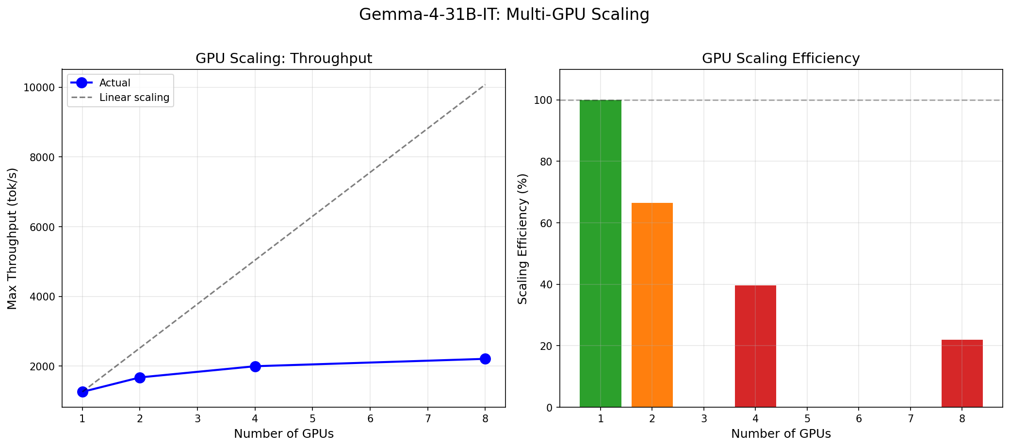
Gemma 4 vs the MoE Field: When a 31B Dense Model Wins and When It Doesn't
Gemma 4 31B scores 9.73/10 MT-Bench from 31B dense params. We compare it against Mixtral 8x22B and DeepSeek V3 on cost, latency, and quality tradeoffs.
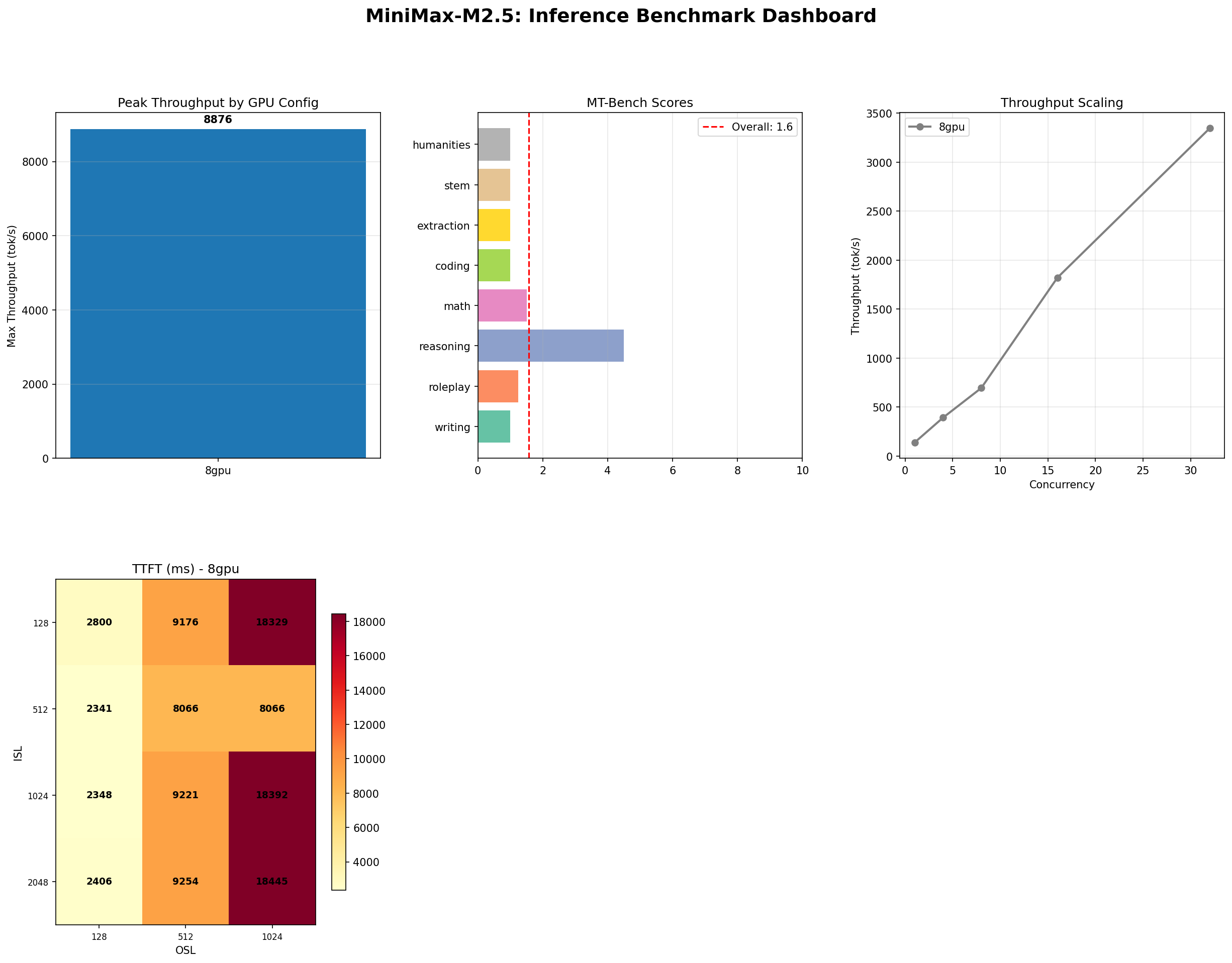
MiniMax M2.5: A 229B MoE Model That Defies Easy Judgment
MiniMax M2.5 229B MoE benchmarked on 8x H100: 8,876 tok/s peak, 100% needle-in-haystack, 87% tool use, but 1.57/10 MT-Bench. The full contradictory picture.
NVIDIA Rubin and Vera: The Next GPU Revolution for AI Infrastructure
NVIDIA Rubin brings HBM4, NVLink 6, and 2x Blackwell performance. Paired with the Vera ARM CPU, it reshapes AI inference economics for every cloud and datacenter operator.